Mapping Vector Data in R
Tufts Data Lab Workshop Spring 2017
Aishwarya Venkat
Data Lab Assistant
Welcome!
Expected previous knowledge:
RStudio basics (data frames, installing packages)
GIS basics (projections, attribute tables)
Why use R to make maps?
Automation/loops for downloading multiple datasets
More control over styles and symbology
Streamlined workflow (sometimes)
Outline
Review spatial data structures
Download shapefile from web, map world population
Map access to water around the world using World Bank's World Development Indicators (WDI) database
Map 2012 state population using choroplethr package
Make county-level choropleth map of household income in USA using American Community Survey (ACS) data
Goals
Become familiar with spatial data structures and sources
Translate geospatial methods (projections, symbology, legends, attributes) to R
Make pretty and informative maps :)
Step 1: Get set up
- Install packages:
packages<-c("choroplethr", "choroplethrMaps", "acs", "WDI", "gstat")
install.packages(packages)
- We will also use pre-installed packages sp, rgdal, dplyr, and ggplot2 during this session
packages<-c("choroplethr", "choroplethrMaps", "acs", "WDI", "sp", "rgdal",
            "ggplot2", "gstat", "dplyr")
lapply(packages, require, character.only = TRUE)
Overview of Spatial Data Structures in R
- Data frames are similar to attribute tables in GIS
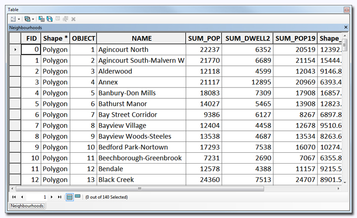
Overview of Spatial Data Structures in R
Each feature in attribute table is associated with discrete spatial information (point, line, or polygon)
Vector data = points, lines, polygons (package: sp)
- Points: SpatialPoints, SpatialPointsDataFrame
- Lines: SpatialLines, SpatialLinesDataFrame
- Polygons: SpatialPolygons, SpatialPolygonsDataFrame
Raster data = pixel/gridded data (packages: rgdal, raster)
- Rasters, raster stacks/bricks, etc.
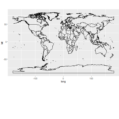
Polygon data: World
Download and map world borders
download.file("http://thematicmapping.org/downloads/TM_WORLD_BORDERS_SIMPL-0.3.zip",
              destfile="world.zip"); unzip("world.zip");
worldmap=readOGR(dsn= getwd(), layer="TM_WORLD_BORDERS_SIMPL-0.3")
ggplot(worldmap, aes(x = long, y = lat, group = group)) + geom_path()+
  theme(aspect.ratio=0.6, plot.margin = unit(c(0, 0, 4, 0), "cm"))
Explore worldmap
- What kind of object is it? What projection is it in? What data does it contain?
str(worldmap)
worldmap@proj4string
str(worldmap@data)
head(worldmap@data)
##   FIPS ISO2 ISO3 UN                NAME   AREA  POP2005 REGION SUBREGION
## 0   AC   AG  ATG 28 Antigua and Barbuda     44    83039     19        29
## 1   AG   DZ  DZA 12             Algeria 238174 32854159      2        15
## 2   AJ   AZ  AZE 31          Azerbaijan   8260  8352021    142       145
## 3   AL   AL  ALB  8             Albania   2740  3153731    150        39
## 4   AM   AM  ARM 51             Armenia   2820  3017661    142       145
## 5   AO   AO  AGO 24              Angola 124670 16095214      2        17
##       LON     LAT
## 0 -61.783  17.078
## 1   2.632  28.163
## 2  47.395  40.430
## 3  20.068  41.143
## 4  44.563  40.534
## 5  17.544 -12.296
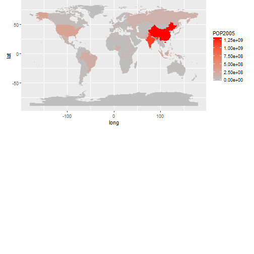
Map 2005 population with ggplot
library(RColorBrewer); library(maptools);

worldmap@data$id=rownames(worldmap@data)
worldmap_points<-fortify(worldmap, region="id")
worldmap_df<-join(worldmap_points, worldmap@data, by="id")

ggplot(worldmap_df, aes(long, lat, group=group, fill=POP2005))+geom_polygon()+
  scale_fill_continuous(low="grey", high="red")+ coord_fixed() +
  theme(aspect.ratio=0.6, plot.margin = unit(c(0, 0, 9, 0), "cm"))
World Development Indicators
Create world map of 2010 Access to water
library(WDI); library(rworldmap);
datamap = WDI(indicator = "SH.H2O.SAFE.ZS", start=2010, end=2010);
SPDF <- joinCountryData2Map(datamap, joinCode = "ISO2", nameJoinColumn = "iso2c");
mapParams <- mapCountryData(SPDF, nameColumnToPlot='SH.H2O.SAFE.ZS', mapTitle="",
             mapRegion="world", catMethod="quantiles", numCats=10, colourPalette='heat');
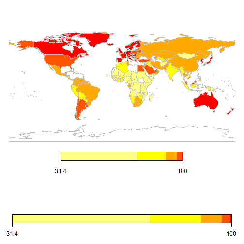
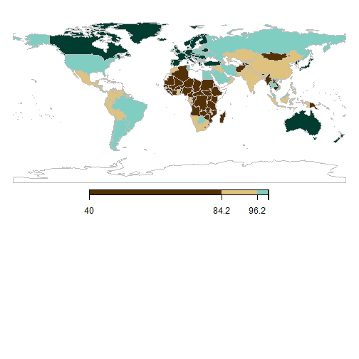
Changing legends and using RColorBrewer scales
cp <- brewer.pal(10,'BrBG')
datamap = WDI(indicator = "SH.H2O.SAFE.ZS", start=2014, end=2014);
SPDF <- joinCountryData2Map(datamap, joinCode = "ISO2", nameJoinColumn = "iso2c");
mapParams <- mapCountryData(SPDF, nameColumnToPlot='SH.H2O.SAFE.ZS', addLegend=TRUE,
             mapRegion="world", catMethod="quantiles", numCats=10, colourPalette=cp, mapTitle = "")
do.call(addMapLegend, c(mapParams,legendLabels="all",legendWidth=0.5,legendIntervals="data",
                        legendShrink=0.5, legendMar = 16))
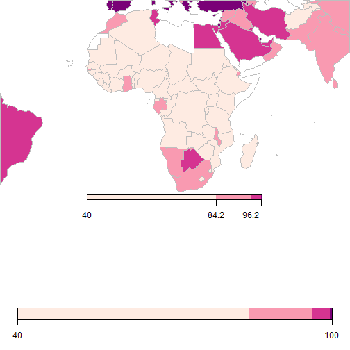
Zooming into Africa
cp <- brewer.pal(5,'RdPu'); datamap = WDI(indicator = "SH.H2O.SAFE.ZS", start=2014, end=2014)
SPDF <- joinCountryData2Map(datamap, joinCode = "ISO2", nameJoinColumn = "iso2c")
mapParams <- mapCountryData(SPDF, nameColumnToPlot='SH.H2O.SAFE.ZS', addLegend=TRUE,
             mapRegion="Africa", catMethod="quantiles", numCats=10, colourPalette=cp)

do.call(addMapLegend, c(mapParams,legendLabels="all",legendWidth=0.5,legendIntervals="data",
                        legendShrink=0.5, legendMar = 15))
American Community Survey data
Load and Explore choroplethR data
library(choroplethr)
library(choroplethrMaps)

data(state.regions)
head(state.regions)
##       region abb fips.numeric fips.character
## 1     alaska  AK            2             02
## 2    alabama  AL            1             01
## 3   arkansas  AR            5             05
## 4    arizona  AZ            4             04
## 5 california  CA            6             06
## 6   colorado  CO            8             08
data(df_pop_state)
head(df_pop_state)
##       region    value
## 1    alabama  4777326
## 2     alaska   711139
## 3    arizona  6410979
## 4   arkansas  2916372
## 5 california 37325068
## 6   colorado  5042853
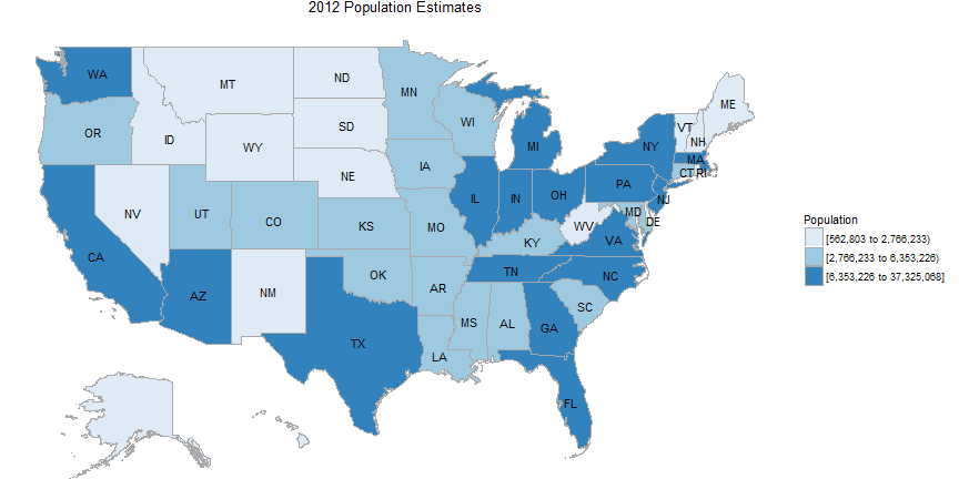
State map of population
state_choropleth(df_pop_state, title = "2012 Population Estimates",
                 legend = "Population", buckets=3)
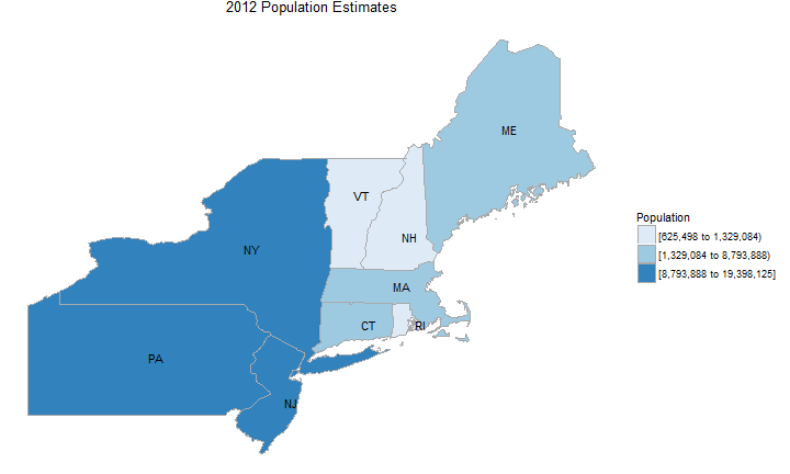
State map of population
state_choropleth(df_pop_state, title = "2012 Population Estimates", legend = "Population",
       buckets=3, zoom=c("connecticut", "maine", "massachusetts", "new hampshire", "vermont",
       "rhode island", "new jersey", "new york", "pennsylvania"))
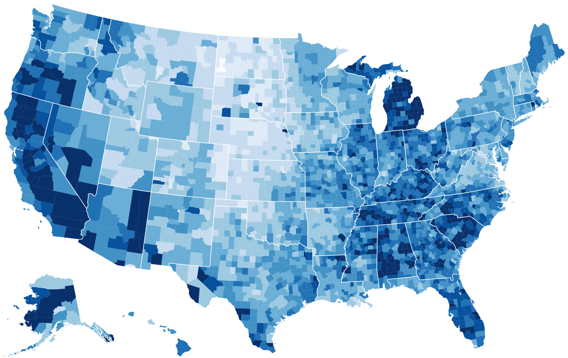
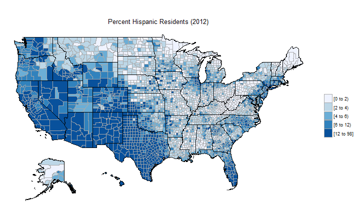
County map of county demographics
data("df_county_demographics")
df_county_demographics$value = df_county_demographics$percent_hispanic
county_choropleth(df_county_demographics, title="Percent Hispanic Residents (2012)", num_colors=5)
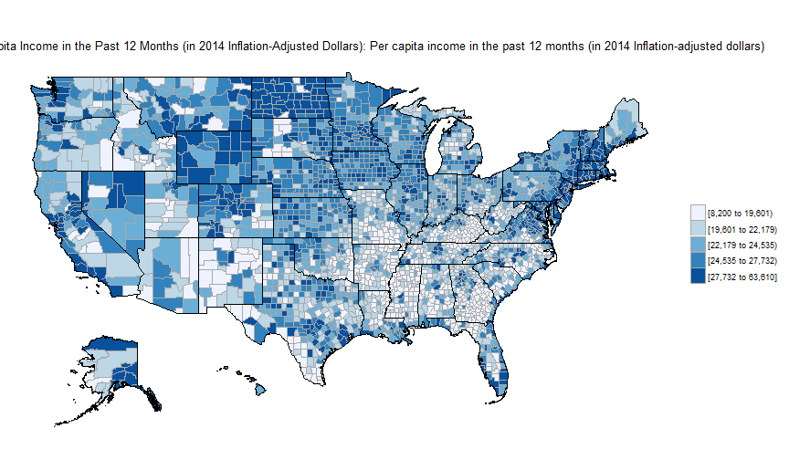
Downloading county-level ACS data
library(acs); api.key.install(key=""); par(mar=c(0,0,0,0), mai=c(0,0,0,0))
county_choropleth_acs("B19301", endyear=2014, span=5, num_colors=5)
Exercises
Exercise 1: Use American Fact Finder to find and map a census variable
query<-acs.lookup(2013, span = 5, dataset = "acs", table.name = "income", case.sensitive=F)
#head(unique(query@results$table.number))
county_choropleth_acs("B01001D", endyear=2013, span=5, num_colors=5)
Exercise 2: Use WDI dataset to map one indicator for a region of your choice
WDIsearch('water'); water = WDI(indicator='SH.H2O.SAFE.ZS', country="all", start=2014, end=2014);
water <- subset(water, !is.na(water$SH.H2O.SAFE.ZS));
water <- group_by(water, country)
water <- filter(water, year == max(year))
names(worldmap_df)[9] <- "iso_a2"
final <- left_join(worldmap_df, water, by="iso_a2")

# Refer to this list for UN regions/subregions designations:
# http://unstats.un.org/unsd/methods/m49/m49regin.htm
# final <- subset(final, REGION==142)

ggplot(final) +
  geom_path(aes(long, lat, group = group), color = "white") +
  geom_polygon(aes(long, lat, group = group, fill = SH.H2O.SAFE.ZS)) +
  scale_fill_gradient("% access to\nimproved water\nsource", low = "#132B43",
                      high = "#56B1F7", na.value = "grey50")
References
Ezra Glenn, Using acs.R to create choropleth maps
Ari Lamstein, Analyzing Census Data in R
Trulia Blog, The choroplethr package for R
Andrew Bonneau, WDI + rworldmap for world map data plotting in Rstudio
Ramnath Vaidyanathan, Slidify presentations from RMarkdown
Advanced examples
Demo dataset: meuse
meuse dataset: concentration of four heavy metals measured in the top soil in a flood plain along the river Meuse, with additional variables
library(sp);
data(meuse); summary(meuse); str(meuse);
##        x                y             cadmium           copper
##  Min.   :178605   Min.   :329714   Min.   : 0.200   Min.   : 14.00
##  1st Qu.:179371   1st Qu.:330762   1st Qu.: 0.800   1st Qu.: 23.00
##  Median :179991   Median :331633   Median : 2.100   Median : 31.00
##  Mean   :180005   Mean   :331635   Mean   : 3.246   Mean   : 40.32
##  3rd Qu.:180630   3rd Qu.:332463   3rd Qu.: 3.850   3rd Qu.: 49.50
##  Max.   :181390   Max.   :333611   Max.   :18.100   Max.   :128.00
##
##       lead            zinc             elev             dist
##  Min.   : 37.0   Min.   : 113.0   Min.   : 5.180   Min.   :0.00000
##  1st Qu.: 72.5   1st Qu.: 198.0   1st Qu.: 7.546   1st Qu.:0.07569
##  Median :123.0   Median : 326.0   Median : 8.180   Median :0.21184
##  Mean   :153.4   Mean   : 469.7   Mean   : 8.165   Mean   :0.24002
##  3rd Qu.:207.0   3rd Qu.: 674.5   3rd Qu.: 8.955   3rd Qu.:0.36407
##  Max.   :654.0   Max.   :1839.0   Max.   :10.520   Max.   :0.88039
##
##        om         ffreq  soil   lime       landuse       dist.m
##  Min.   : 1.000   1:84   1:97   0:111   W      :50   Min.   :  10.0
##  1st Qu.: 5.300   2:48   2:46   1: 44   Ah     :39   1st Qu.:  80.0
##  Median : 6.900   3:23   3:12           Am     :22   Median : 270.0
##  Mean   : 7.478                         Fw     :10   Mean   : 290.3
##  3rd Qu.: 9.000                         Ab     : 8   3rd Qu.: 450.0
##  Max.   :17.000                         (Other):25   Max.   :1000.0
##  NA's   :2                              NA's   : 1
## 'data.frame':    155 obs. of  14 variables:
##  $ x      : num  181072 181025 181165 181298 181307 ...
##  $ y      : num  333611 333558 333537 333484 333330 ...
##  $ cadmium: num  11.7 8.6 6.5 2.6 2.8 3 3.2 2.8 2.4 1.6 ...
##  $ copper : num  85 81 68 81 48 61 31 29 37 24 ...
##  $ lead   : num  299 277 199 116 117 137 132 150 133 80 ...
##  $ zinc   : num  1022 1141 640 257 269 ...
##  $ elev   : num  7.91 6.98 7.8 7.66 7.48 ...
##  $ dist   : num  0.00136 0.01222 0.10303 0.19009 0.27709 ...
##  $ om     : num  13.6 14 13 8 8.7 7.8 9.2 9.5 10.6 6.3 ...
##  $ ffreq  : Factor w/ 3 levels "1","2","3": 1 1 1 1 1 1 1 1 1 1 ...
##  $ soil   : Factor w/ 3 levels "1","2","3": 1 1 1 2 2 2 2 1 1 2 ...
##  $ lime   : Factor w/ 2 levels "0","1": 2 2 2 1 1 1 1 1 1 1 ...
##  $ landuse: Factor w/ 15 levels "Aa","Ab","Ag",..: 4 4 4 11 4 11 4 2 2 15 ...
##  $ dist.m : num  50 30 150 270 380 470 240 120 240 420 ...
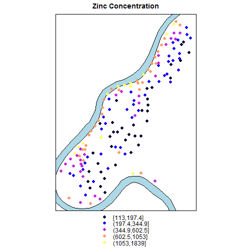
Mapping meuse dataset
coordinates(meuse)=~x+y;

data(meuse.riv);
meuse.sr = SpatialPolygons(list(Polygons(
  list(Polygon(meuse.riv)),"meuse.riv")))
rv = list("sp.polygons", meuse.sr,
          fill = "lightblue")

spplot(meuse["zinc"], do.log = TRUE,
    key.space = "bottom",
    sp.layout = list(rv),
    main = "Zinc Concentration")
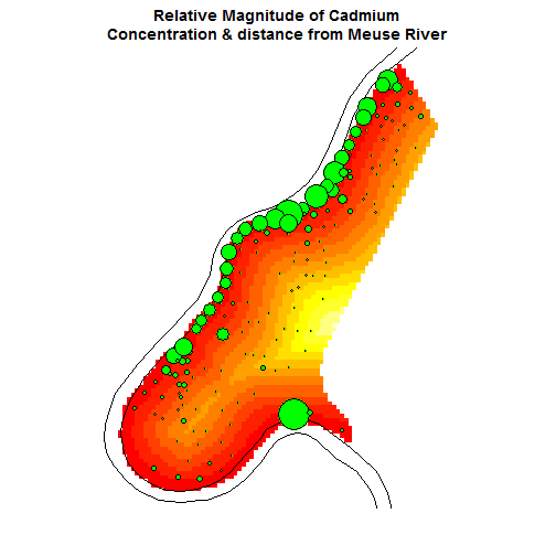
Use spplot to overlay data
data(meuse.grid); coordinates(meuse.grid) = ~x+y;
gridded(meuse.grid) = TRUE

meuse.sl = SpatialLines(list(Lines(list(Line
    (meuse.riv)), ID="1")))

par(mar=c(7,0,4,4));
image(meuse.grid["dist"], main = "Relative Magnitude
of Cadmium Concentration & distance from Meuse River");
lines(meuse.sl);

with(meuse, symbols(x=meuse@coords[,1],
  y=meuse@coords[,2], circles=meuse@data$cadmium,
  inches=1/5, col="black", bg="green", add=T))
Simple interpolation of zinc concentrations
## [inverse distance weighted interpolation]
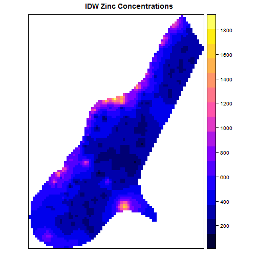
library(gstat)
data(meuse); data(meuse.grid);
coordinates(meuse.grid) = ~x+y;
gridded(meuse.grid) = TRUE

zinc.idw = idw(zinc~1, meuse, meuse.grid)

spplot(zinc.idw["var1.pred"],
       main = "IDW Zinc
       Concentrations")
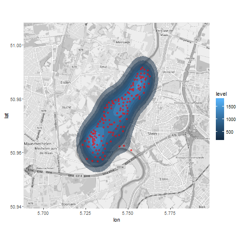
Point density for meuse dataset
library(ggmap); proj4string(meuse) <- CRS("+init=epsg:28992");
meuse_wgs84<-spTransform(meuse,  CRS("+init=epsg:4326"))

meuse_wgs84<-data.frame(meuse_wgs84@coords)
meuse_wgs84$copper<-meuse$copper

map <- get_map(c(lon=mean(meuse_wgs84$x), lat=mean(meuse_wgs84$y)), zoom=13, source = "osm",
               color = "bw"); mapPoints <- ggmap(map)
mapPoints +
  stat_density2d(data=meuse_wgs84,aes(x, y, fill= ..level..), alpha =0.5, geom="polygon") +
  geom_point(data=meuse_wgs84,aes(x, y), colour="red", alpha = .5)
Point density for meuse dataset